This release features biosequence searching, Bioscape, and Chemscape.
STNext now has a streamlined interface to sequence search that:
Simplifies your access to the algorithms you need and the parameters that control them.
Provides sequence search results with alignment and relevant patent information.
Supports dynamic sorting and filtering of results.
Enables crossover from biosequence results to CAPlus and other document databases.
Supports export of results to Excel for collaboration, reporting, and sharing.
There are currently three search modalities supported:
BLAST – A set of local alignment algorithms (BLASTn, MegaBlast, BLASTp, tBLASTn, BLASTx) for searching proteins as well as nucleotides
CDR - For antibody and t-cell receptors
Motif - Enables additional variability in queries to search for short patterns in DNA, RNA, or proteins
There is also comprehensive content containing CAS-curated Registry sequence data and millions of additionally extracted patent sequences from (US, EP, WO, CA, KR, JP, and CN) major patent offices. This new content set contains:
More than 580 million patent sequences from more than 1.1 milion patents and 60+ patent authorities.
Manually curated sequences not found in electronic sequence listings and other databases.
An antibody and t-cell receptor-specific content set containing more than 10 million CDRs.
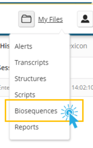
Clicking Biosequences in the My Files menu will take you to the main sequence search interface.
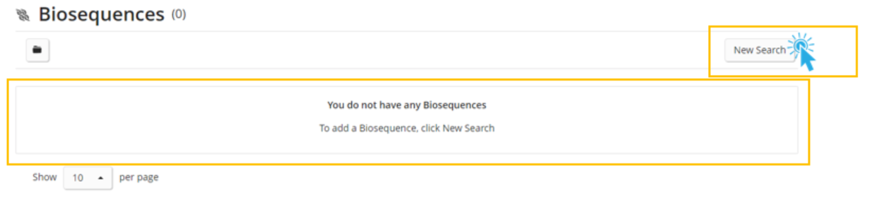
The Biosequences page has a search history and any running or completed searches. The first time a user accesses this area, they will have no previously run or currently running searches; there will only be the option to create a new search.
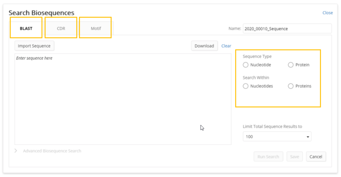
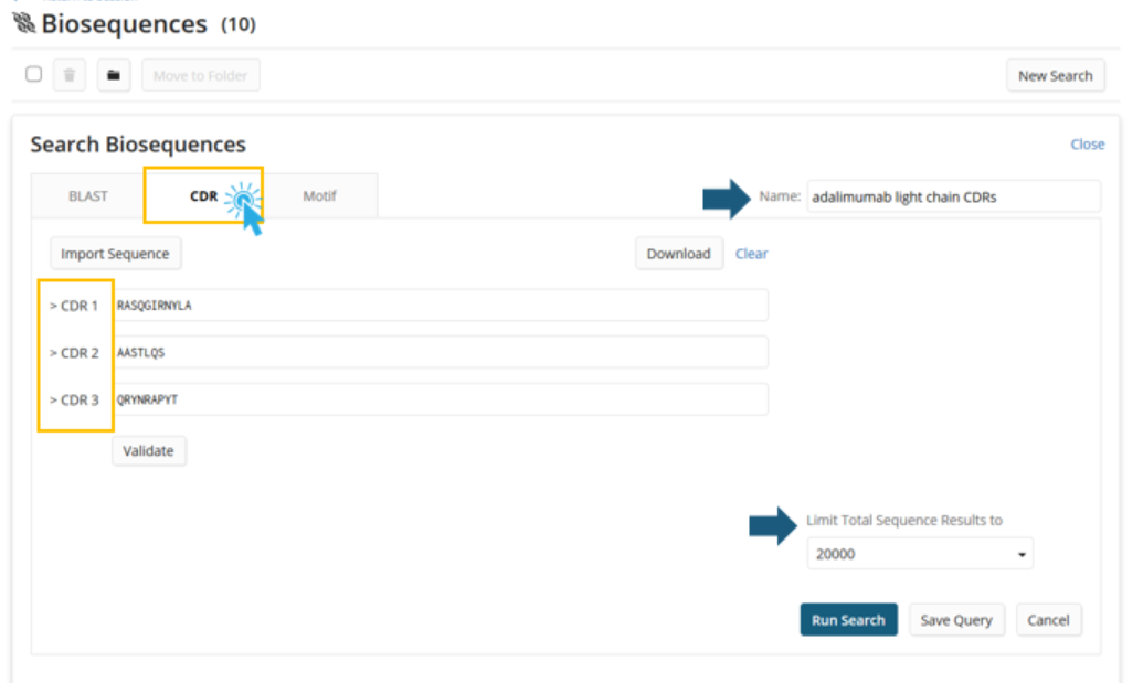
After clicking the New Search button, a user is presented with an interface to enter their query. Three search modalities are currently available: BLAST, CDR, and Motif.
Basic Local Alignment Search Tool (BLAST) is designed to find local, rather than global, alignments. Its heuristics are based for speed and it has been continually developed at the NCBI for 20+ years. There are a number of BLAST algorithm variants provided in the interface. The algorithm used is dictated by the user’s selection of the type of sequence searching they would like to perform.
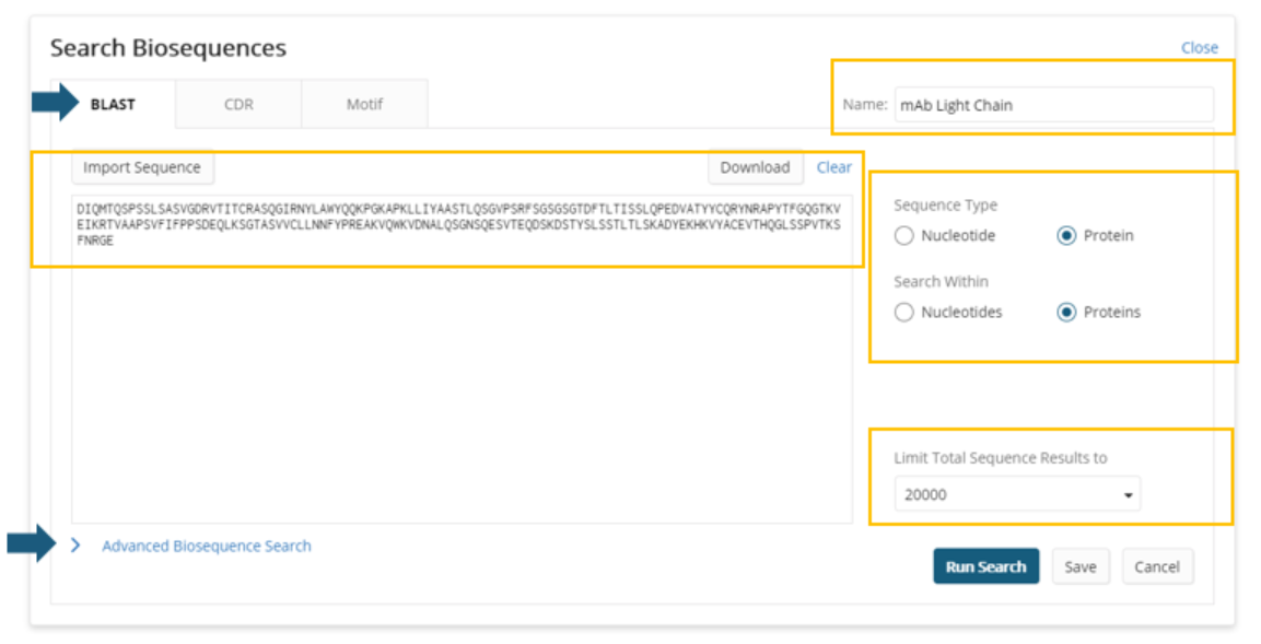
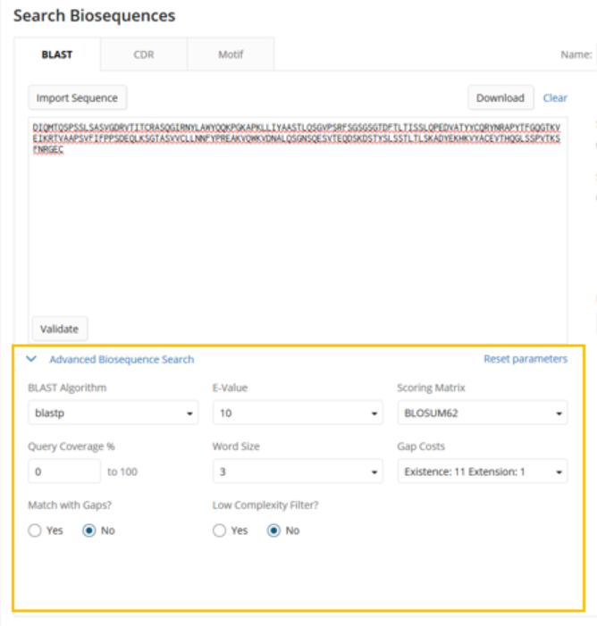
On the BLAST tab, a user can enter their query, select their search type and the type of sequences they’d like to search against, and name their search to provide a useful title for their result set.
For BLAST searching, there is an expansion of the maximum number of results that can be returned from a search. Large answer sets may require longer processing time. With that in mind, Advanced Biosequence Search parameters are provided to tune the performance of the search.
The advanced parameters can be used to:
Increase the speed of the search.
Adjust for the length of the query sequence.
Tune
the sensitivity of the search for finding sequences that are more
distantly related to the query or finding nearly exact sequences.
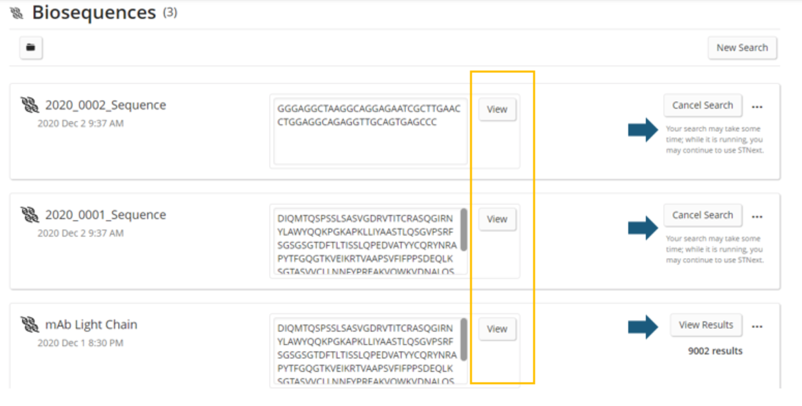
Due to the nature of the algorithms, the execution of a search may take anywhere from several seconds to several minutes. Thus, the search is performed asynchronously. Upon submitting a search, the user will be taken to their search history where they can see the status of any currently running searches, cancel a currently running search, or access the results from completed searches.
A user can also view a previous query and the parameters that were used, edit the query or parameters, and then save and run the search with updated settings.
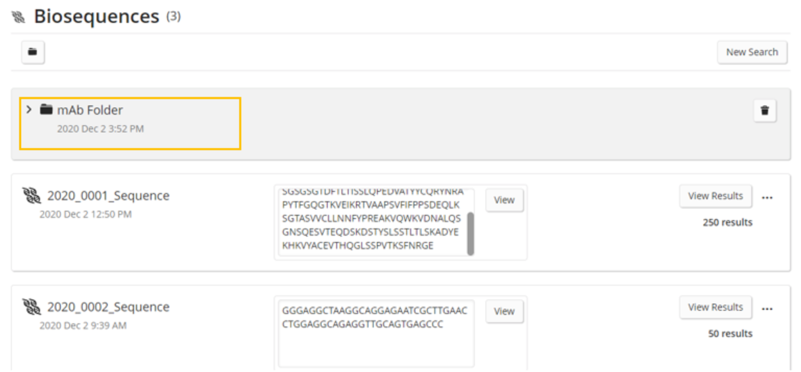
Clicking the ellipsis to the right of the View Results button opens a menu that allows the answer sets to be managed. The current options are delete or move.
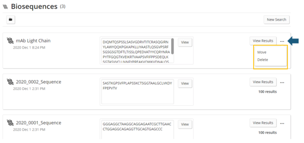
Selecting the Move option allows a user to move their query and accompanying result set into a folder to assist with organizing all of the searches related to a given project.
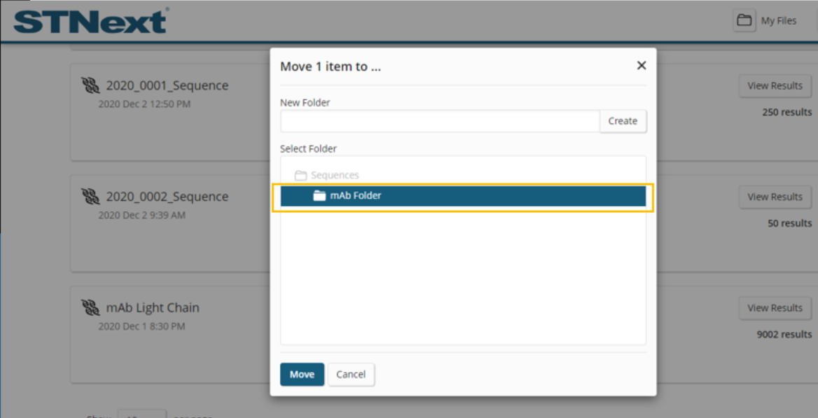
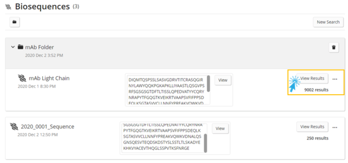
Once a query/answer set has been moved into a folder, the folder can then be expanded to reveal the answer sets and query parameters within.
The user can now click the View Results button for a particular answer set.
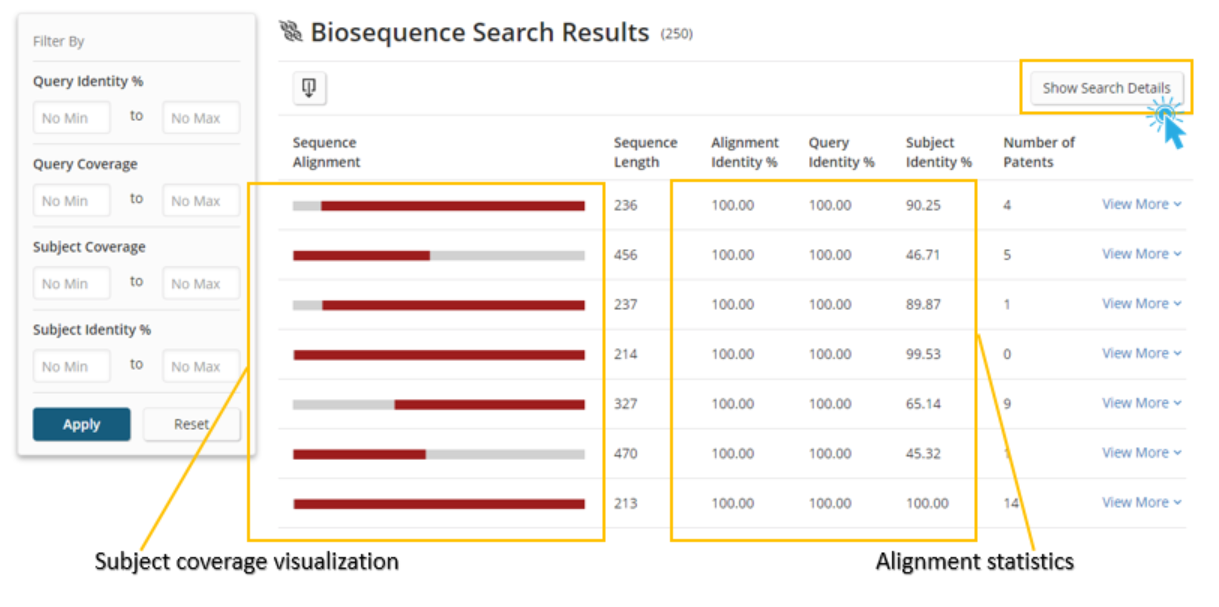
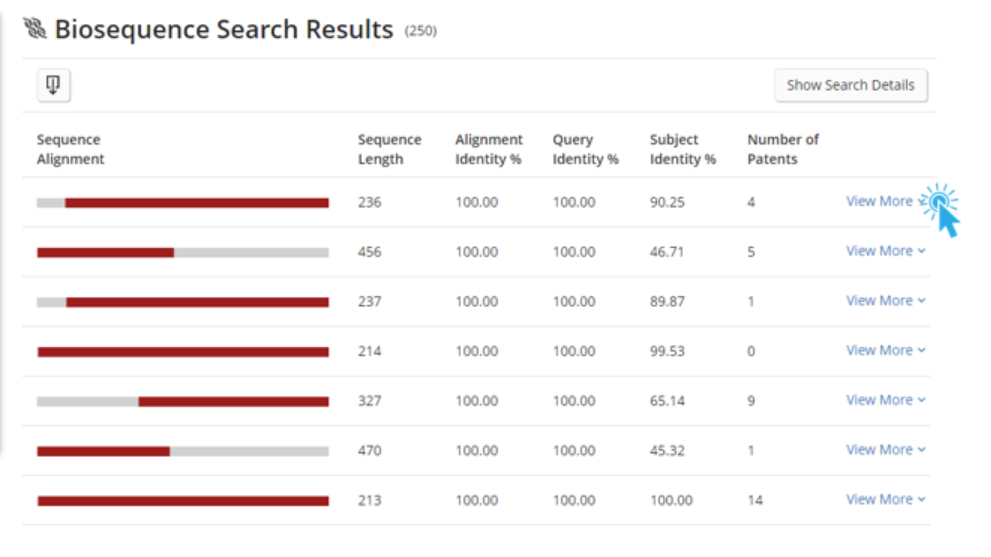
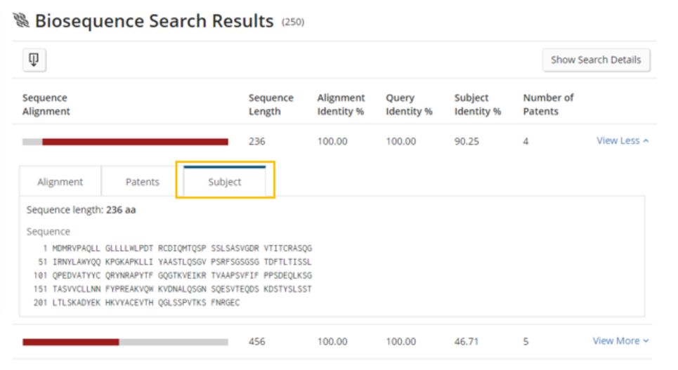
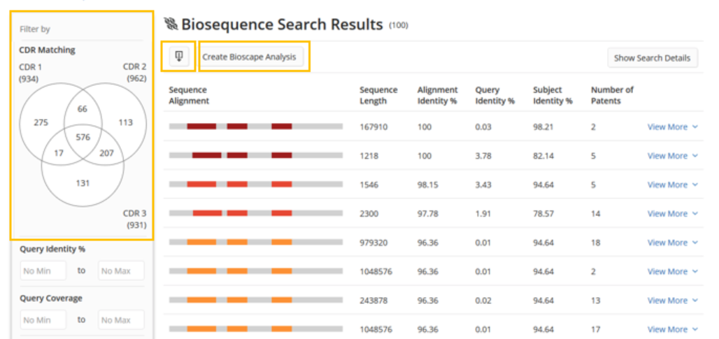
After clicking the View Results button, the user is taken to a tabular view of the results, where they can quickly and easily see a visualization of the subject coverage and the key statistics for assessing the quality of the alignments. On the left panel, there are range filters to narrow the results based upon the alignment statistics that are most relevant to the user.
To understand the query and parameters that led to this answer set, the user can click the Show Search Details button.
After clicking the Show Search Details button, an information panel above the results table expands.
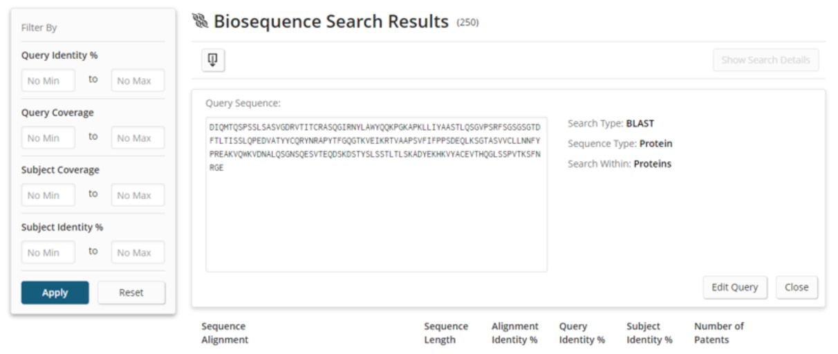
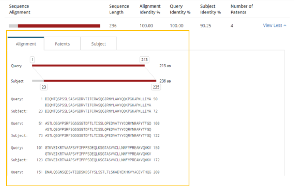
Clicking View More displays a more detailed view of the alignment, references, and subject data.
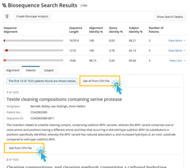
The user has access to information about the documents in which the subject sequence occurs. From here, they can click the Get All from STN File button to crossover to a document file and search all of the references associated with that sequence or click the Get from STN File button for a single document to crossover and search for that particular reference.
After clicking the Get All from STN File or Get from STN File buttons, the user is presented with a choice of STN files to cross over into.
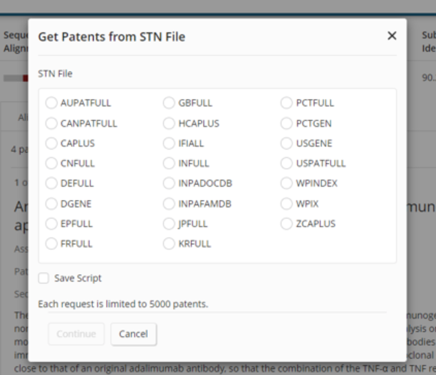
After selecting a file, the user is taken to that file to access more document details and create subsets using keyword searching.
Back within the sequence results, a user can also access sequence level details of the subject (hit) sequence to which their query aligned.
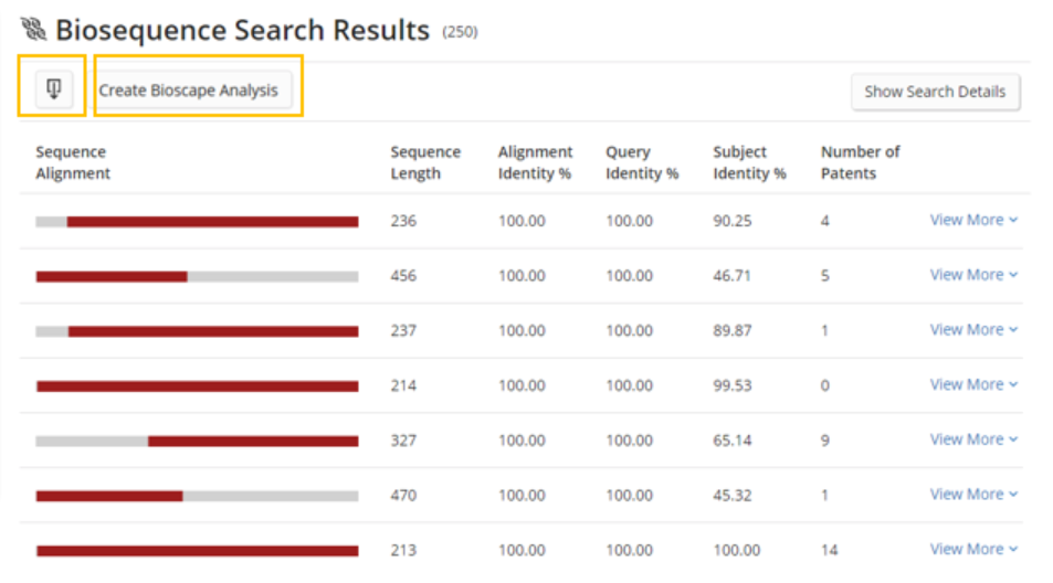
Finally, a user can export the answer set to an Excel format (.xls) file that contains the alignments, patents in which the sequences were found, and relevant identifiers for the sequences such as the seq id number used by each patent and the associated CAS registry numbers.
Note: Not all sequences will have registry numbers.
The answer set can also be visualized by clicking the Create Bioscape Analysis button, which will be discussed in the Bioscape section.
Complimentarity Determining Regions (CDRs) can be thought of as substrings of the overall sequence important to the functionality of the antibody. Here, highlighted in orange, you can see the CDRs on the light chain of the ABBVIE blockbuster drug Humira®.
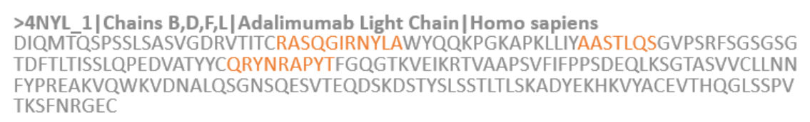
Each chain of an antibody has three CDRs, which can make antibody searching particularly challenging.
CDR search allows a user to simultaneously search three CDRs. For a CDR search, there are no advanced parameters like the BLAST search. The parameters have been optimized for the CDRs' short sequence length to provide the most relevant results.
However, similar to the BLAST search interface, there is the ability to adjust limits on the number of answers and name the search/answer set.
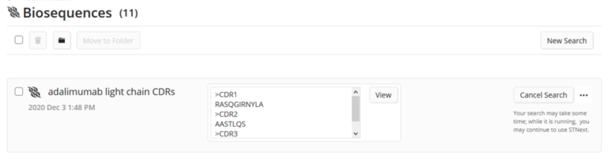
After running a CDR search, similar to the BLAST search, the user is taken to their search history where they can see result sets from previous searches and currently running searches.
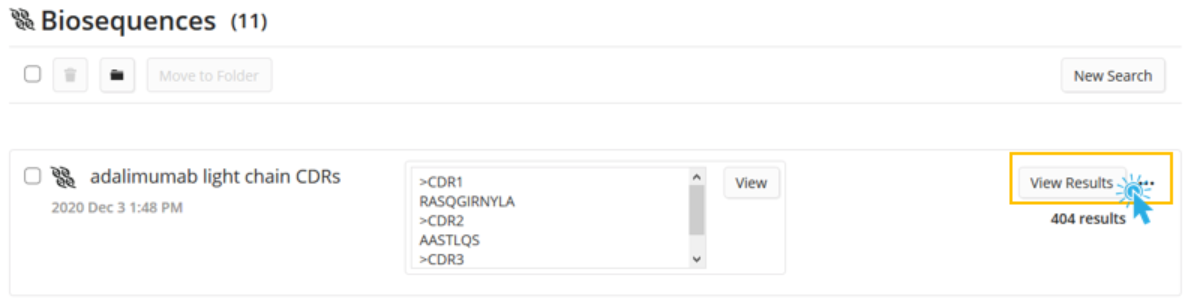
Upon completion of the search, the user can then click the View Results button.
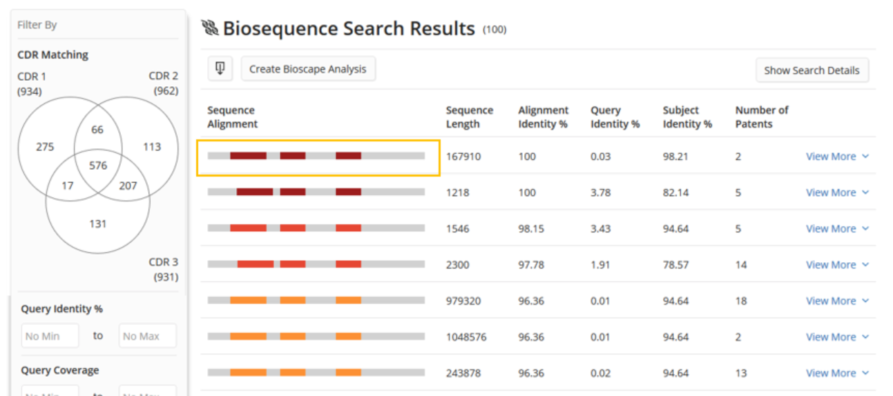
The user will again see results very similar to the BLAST answer set. The key differences will be that in the ideal CDR alignment visualization, there will be three color bands that correspond to alignment of each of the three CDRs in the user’s query.
For example, in the first result, we see three red bands that correspond to alignments of the three query sequences.
Clicking View More and expanding the Alignment tab provides additional detail on the alignments.
Again, this is comparable to the BLAST example except that there will be up to three sets of alignment details displayed: one for each aligned CDR in the query.
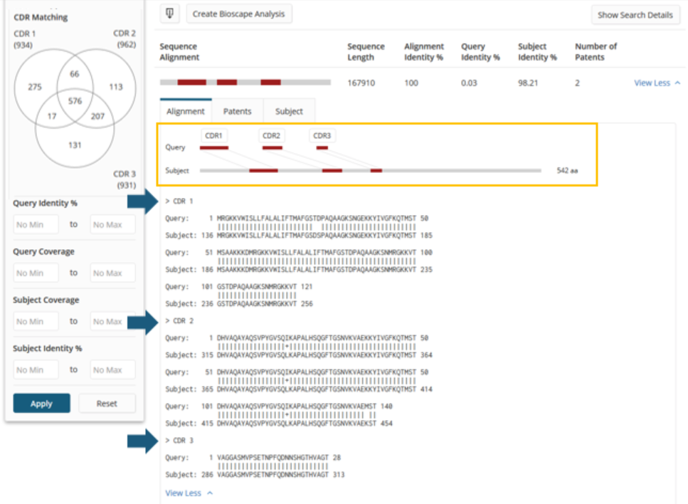
Of course, it is also possible that the search has resulted in some sequences that contain only one or two of the CDRs from the query.
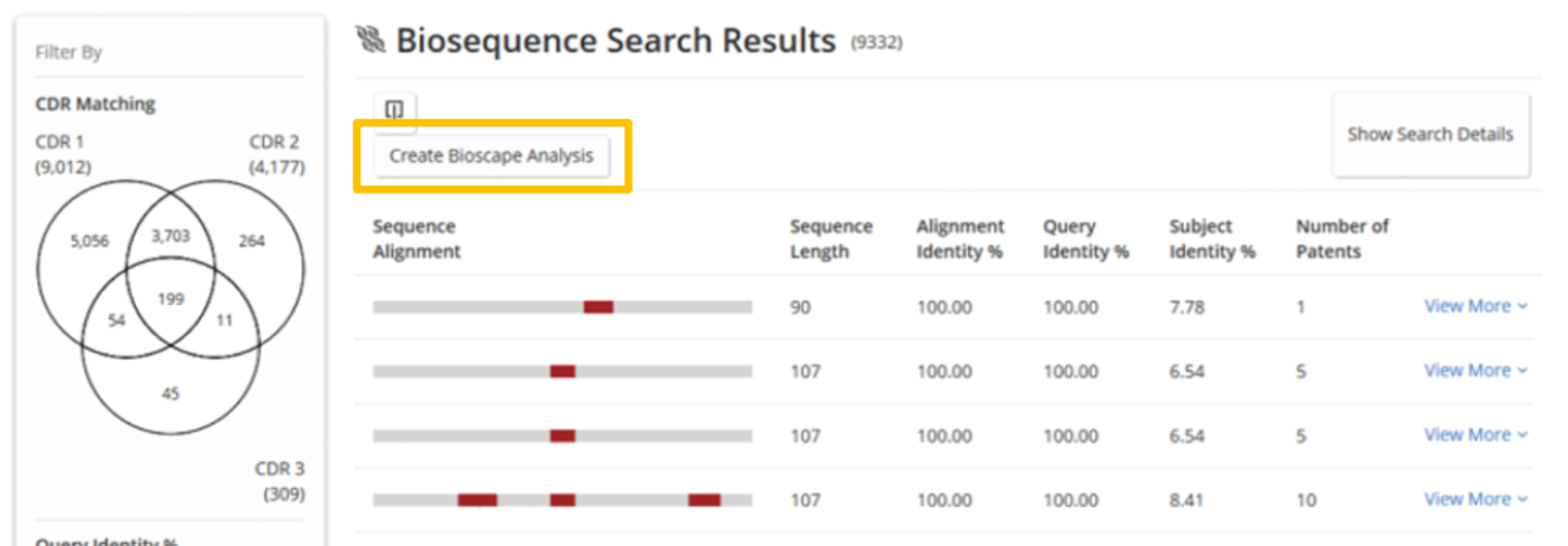
This is where the CDR results again differ from BLAST. The filters area now contains a Venn diagram that allows users to filter the results to those containing all three CDRS or any of the possible combinations of alignments with numbers to indicate the amount of results in each subset.
Features such as export and Bioscape visualization are also available here as in BLAST.
Motif is a search modality that allows for the searching of patterns within a sequence.
For instance, Lilly and Precision Biosciences have recently announced a genome editing research collaboration based upon Precision Biosciences’ DNA-cutting enzymes derived from a family of enzymes that share a common conserved pattern shown here.
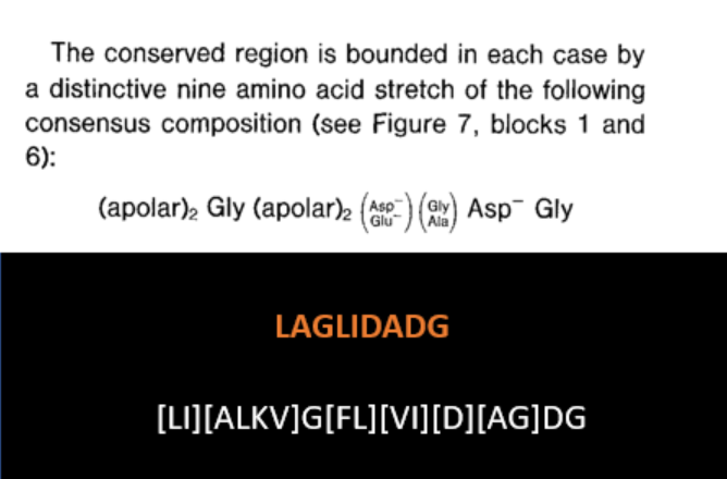
The family of proteins goes by the name shown in orange which is a common variation of that conserved pattern.
A potential motif search query to find related sequences is also shown with bracketed letters representing various substitutions that can occur at a single position.
A note about motif search: The motif search within our new interface is considerably different than the motif search supported from the command line of Registry. Command line Registry motif search acts similar to a regular expression search. However, this new implementation is a motif enumerator, in which the pattern is expanded to discrete search terms and queried with BLAST.
This allows the search to be performed quickly using BLAST’s heuristic nature and allows for extra variability in the matched sequences due to the probabilistic nature of the BLAST algorithm. A trade off however, is that the number of enumerations possible is limited and can result in a query that reaches system limits. It also means the “+” and “*” operators are not supported in this modality as they can not be exhaustively enumerated into search terms.
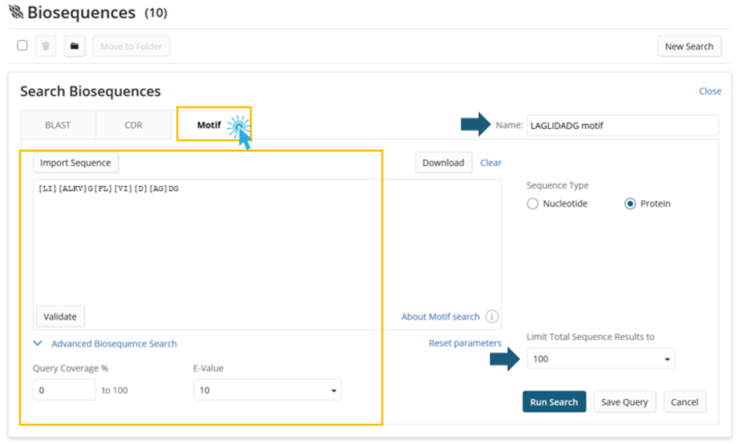
As with BLAST and CDR search, the user may assign a name to their query/answer set and adjust the maximum answer set size to their needs.
The user will also need to specify the type of sequence that they are using as a query (as they do in BLAST) and will have access to a limited set of advanced options available for tuning the level of matching performed.
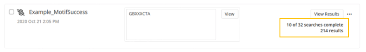
Because the motif search enumerates the pattern into individual search terms, a motif result set will indicate the number of enumerated searches being performed and any that have completed.
After clicking the View Results button, the user views the results page, which is similar to a BLAST search results page with a notable exception: the Query Sequence drop-down menu.
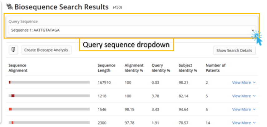
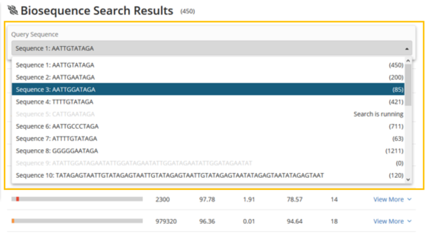
The drop-down menu provides access to the results of each enumeration of the motif pattern. Selecting any of the enumerated queries displays the results of that query. Besides the Query Sequence drop-down menu, motif results appear exactly as they do for BLAST.
This feature allows users to visually explore patents around sequences returned as part of sequence search results.
A visualization of the first 1000 sequence results can be created by clicking the Create Bioscape Analysis button.
The position of the sequences in the Bioscape display represent the relative similarity of their alignment to the query. Proximity in Bioscape does not necessarily indicate that two sequences are similar, only that the nature of their alignment to the query is similar. Thus, sequences that are similar to one another may not be adjacent to one another in Bioscape if the nature of their alignment to the query is significantly different.
Accordingly, dissimilar sequences that share similar alignment to the query would be expected to be within close proximity of one another. The final layout is a best fit when considering the overall similarity or dissimilarity of all sequences from the result set.
For BLAST and Motif searches, the query sequence is denoted with a blue circle. For simplicity, no blue highlighting is presented for CDR searches (which are a combination of similarity/dissimilarity across three regions).
The color of each sequence on the graph represents the percentage of identical matches of that sequence compared to the query sequence for the alignment between the two.
The height represents the number of patents that reference a given sequence
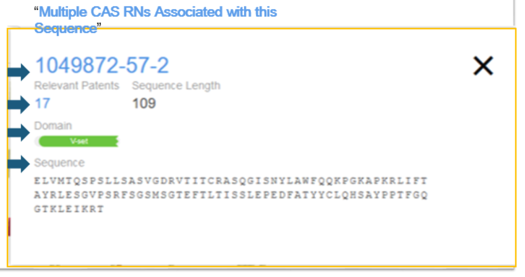
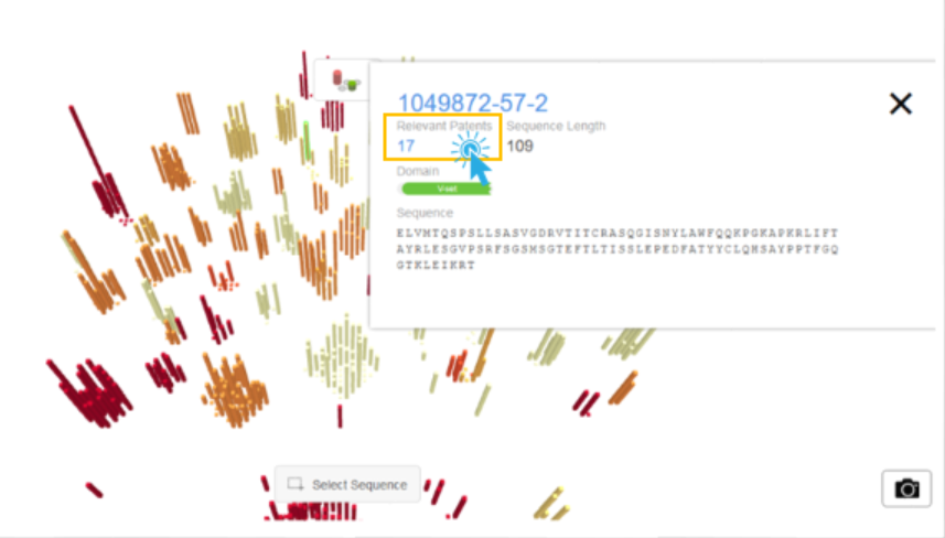
More information about each sequence can be seen by clicking its bar. A window on the right then displays with the following information:
Registry information if available
The number of patents referencing the sequence
The domain if available
The sequence
Note that for registry information:
If a single registry number is associated with the sequence, it is displayed.
If multiple registry numbers are associated with the sequence, the text Multiple CAS RNs Associated with this Sequence displays.
If no registry number is associated with the
sequence, no registry information displays.
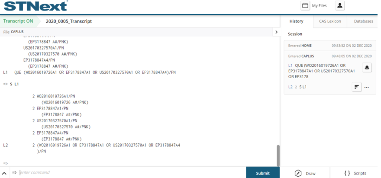
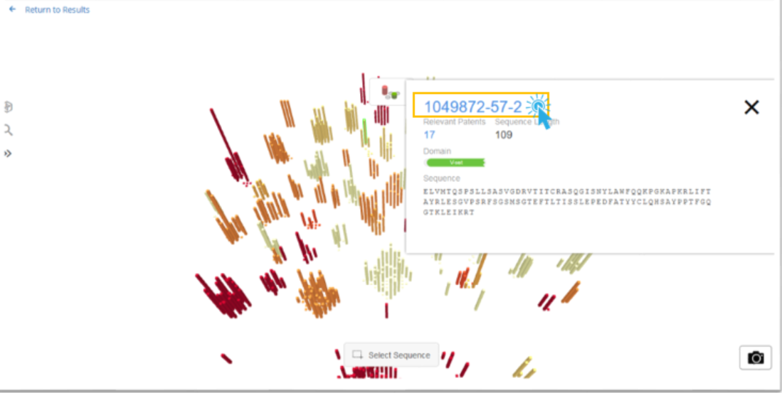
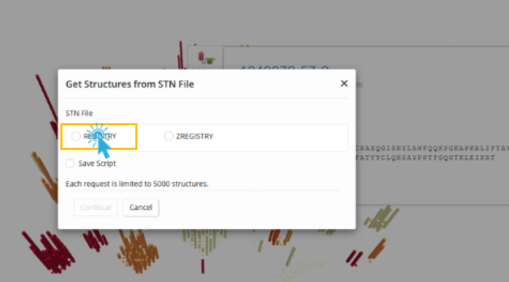
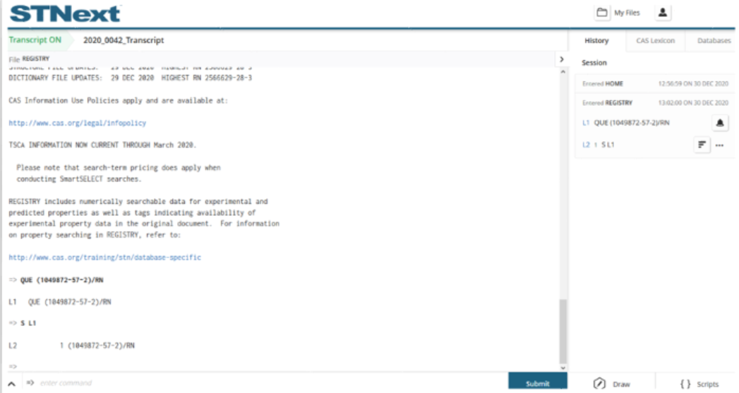
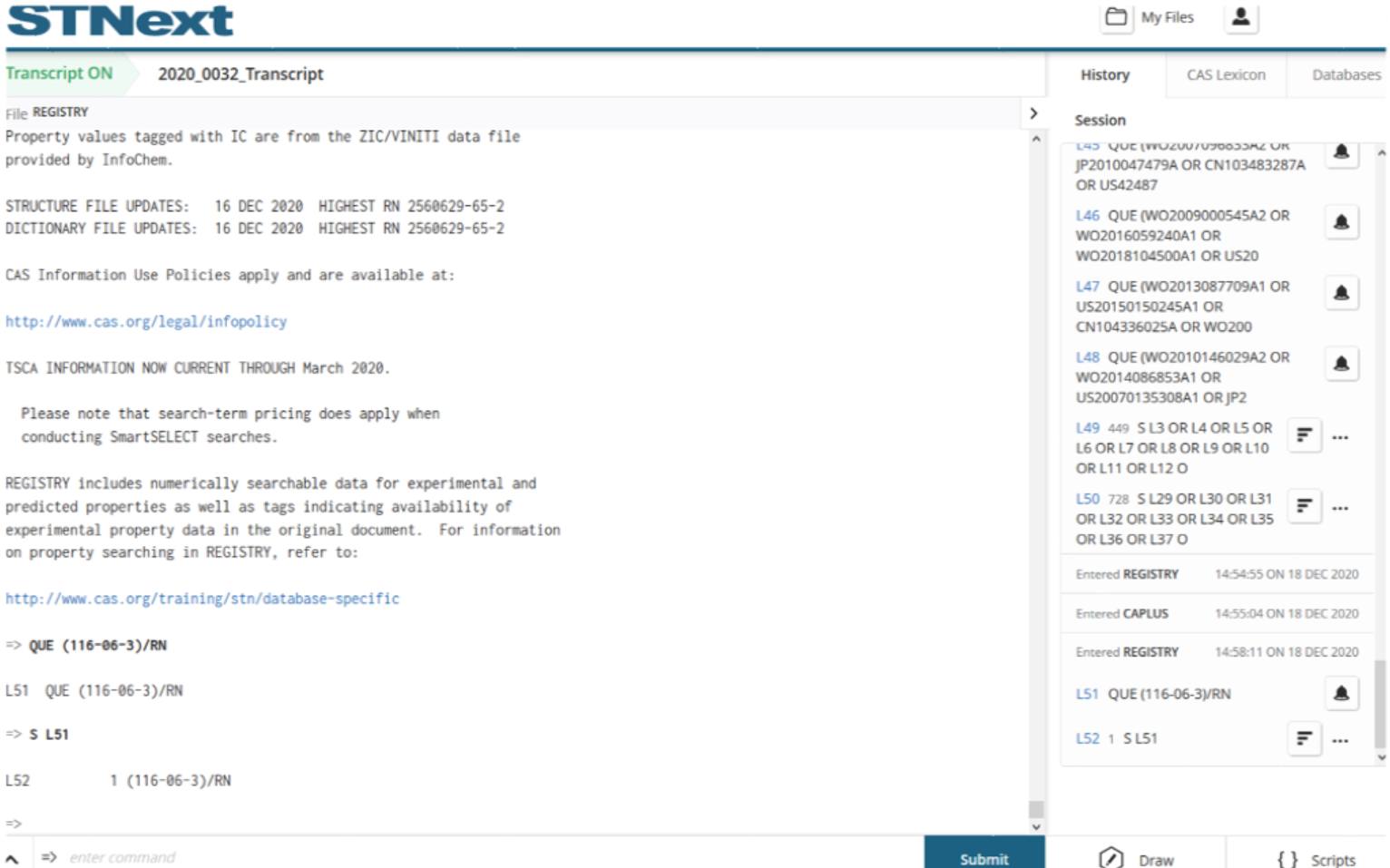
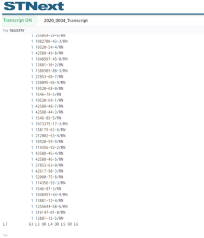
When an RN or the text Multiple CAS RNs Associated with this Sequence displays, the user can click those links to create a search containing the related substances. For example, when we click on the displayed registry number, we are presented with a choice for which file to use for the crossover.
We choose REGISTRY for this example and click Continue.
We are then presented with the search results for the related substance.
Users can also gain further insight into patents referencing a given sequence by clicking the blue patent count. This performs a search using the related patents, allowing the user to further explore those patents. For example, when we click the patent count for this sequence, we are presented with a choice of which file to use for the crossover.
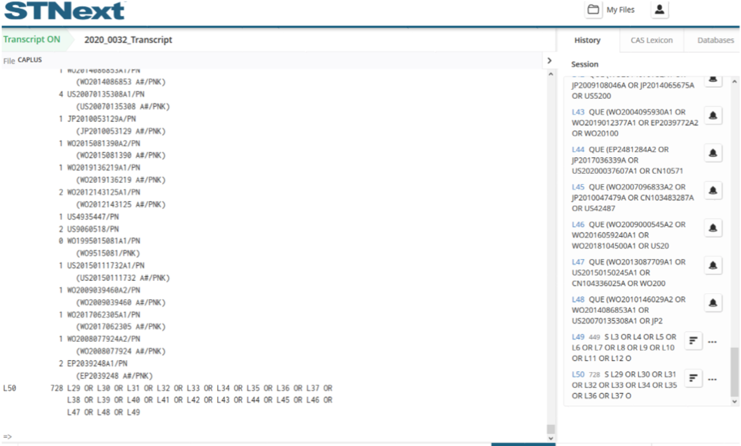
We choose CAPLUS for this example. Note this search will be limited to the first 5000 patents
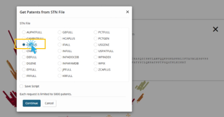
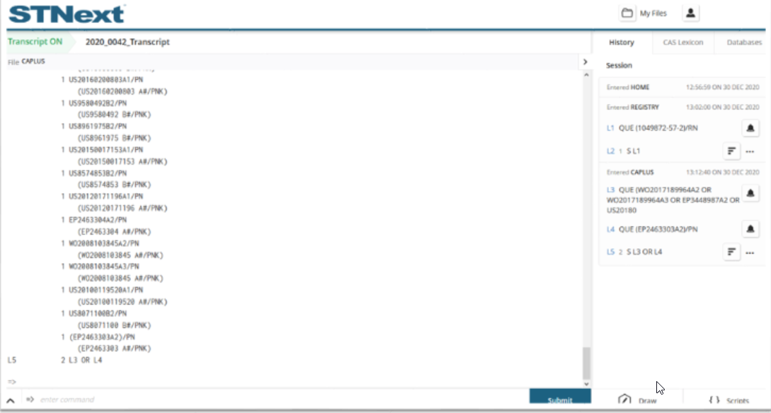
We are then then presented with the search results for the related set of patents.
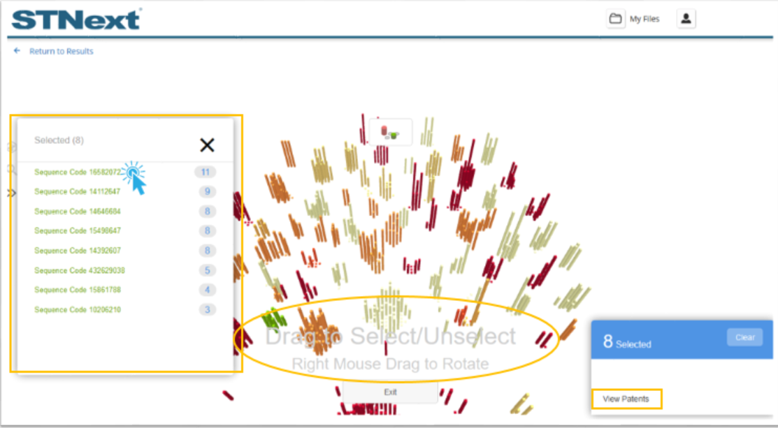
Users can also select a set of sequences from the visualization in order to review details about each, view patents related to individual sequences, or view patents related to the range of selected sequences.
This is done by clicking the Select Sequence button at the bottom of the visualization. Users can then click and drag around target sequences.
From here, users can click any of the items in the presented list to get the detail window. They can also click the circled number for any item in the list to get the patents for the related sequence or they can click the View Patents button in the lower-right corner to view the patents for all selected sequences.
The Find tool found on the left of the visualization may be used to locate sequences by text and/or simple legal status found in patents which reference a given sequence.
For the example, a user could search for ‘cancer’ and ‘Active’ and ‘Pending’ legal status.
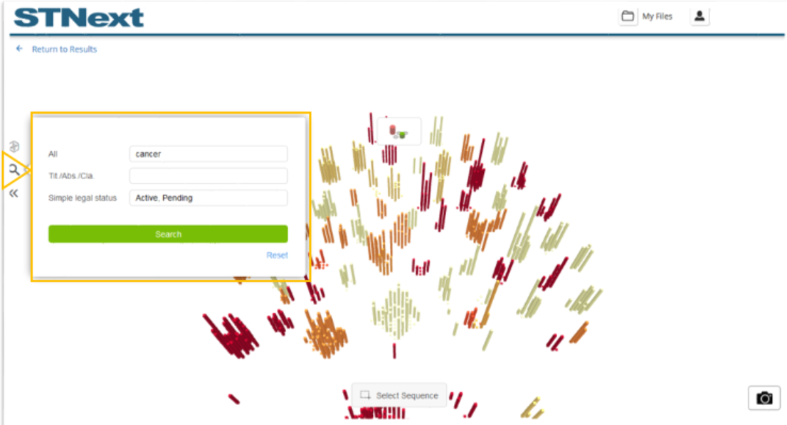
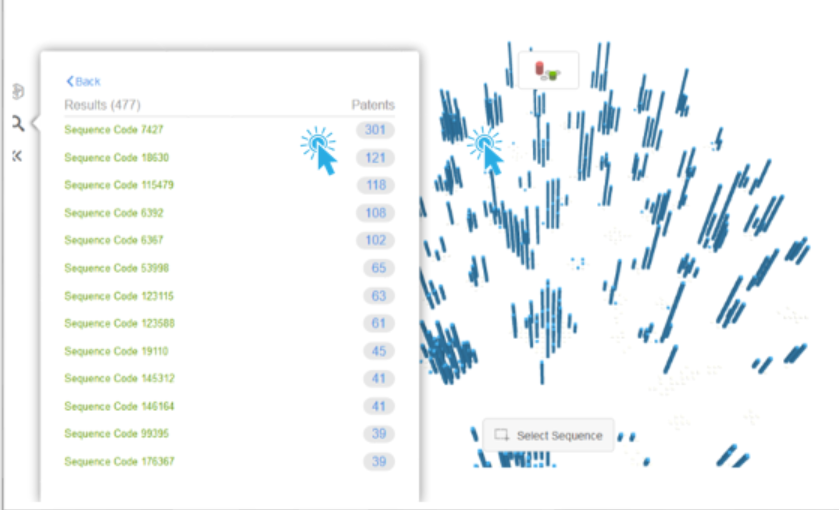
This will then display a list of related sequences and update the visualization to only show those sequences in blue. Users can then click the list or visualization to further explore the related sequences.
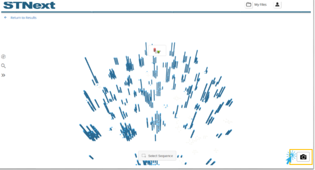
Users can also save a screenshot of the current visualization by clicking the camera icon in the lower-right corner. A screenshot is then downloaded to the browser.
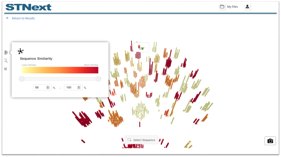
Users can also change how the visualization is presented. By default, Bioscape only shows highlighted sequences.
This can be helpful to focus on selected items, but it can also be helpful to see the other sequences for context.
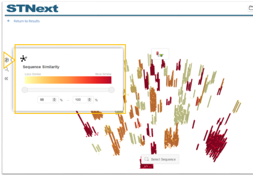
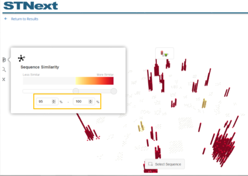
To show this in action, the similarity can be adjusted by selecting the uppermost icon on the left. In the example, the minimum similarity was adjusted to 95%. Doing something like this can be helpful to further focus on higher similarity sequences. Note the coloring is adjusted to the new range.
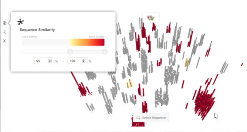
To further show how the view can be changed to include sequences not selected by the current filter, the view selector could then be set to All Sequences.
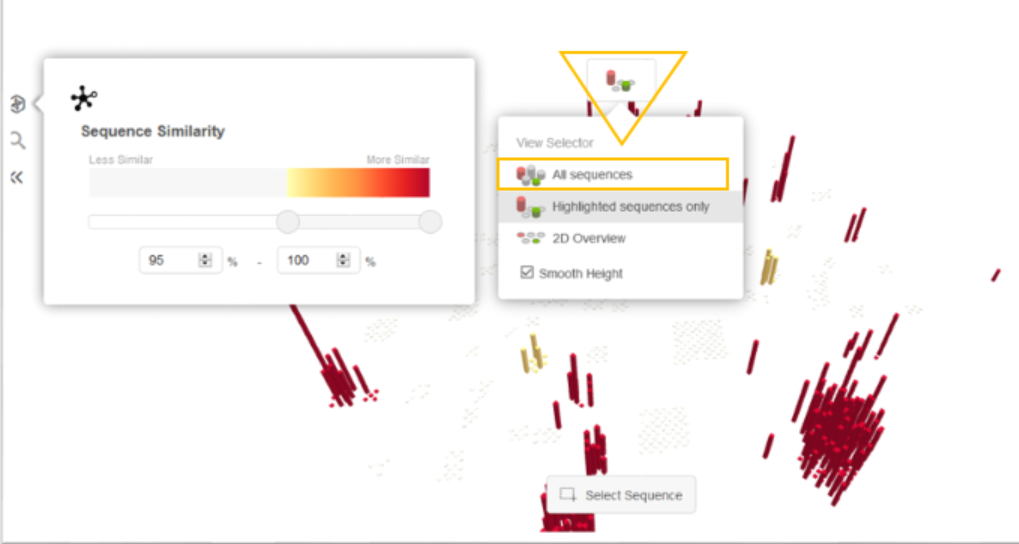
These sequences are now displayed in gray.
Chemscape allows users to visually explore patents for a structure search result set that is based on a drawn structure.
For example, if we wanted to explore substances around a banned pesticide, aldicarb (116-06-3), we could draw the structure or generate it from the registry number, and then perform a substructure search.
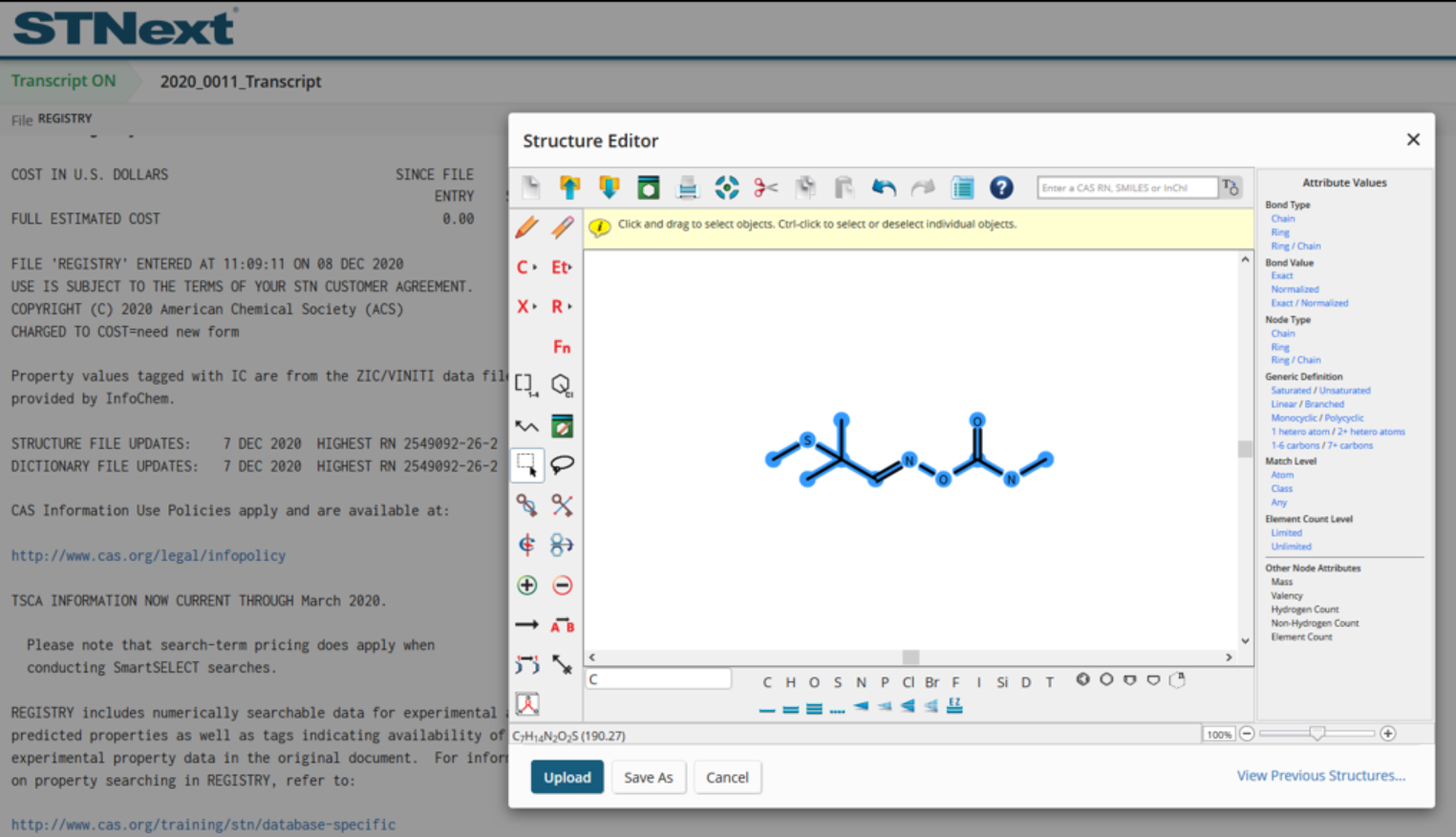
The option to generate a Chemscape visualization is found in the ellipsis (...) menu next to the L number associated with the substructure search.
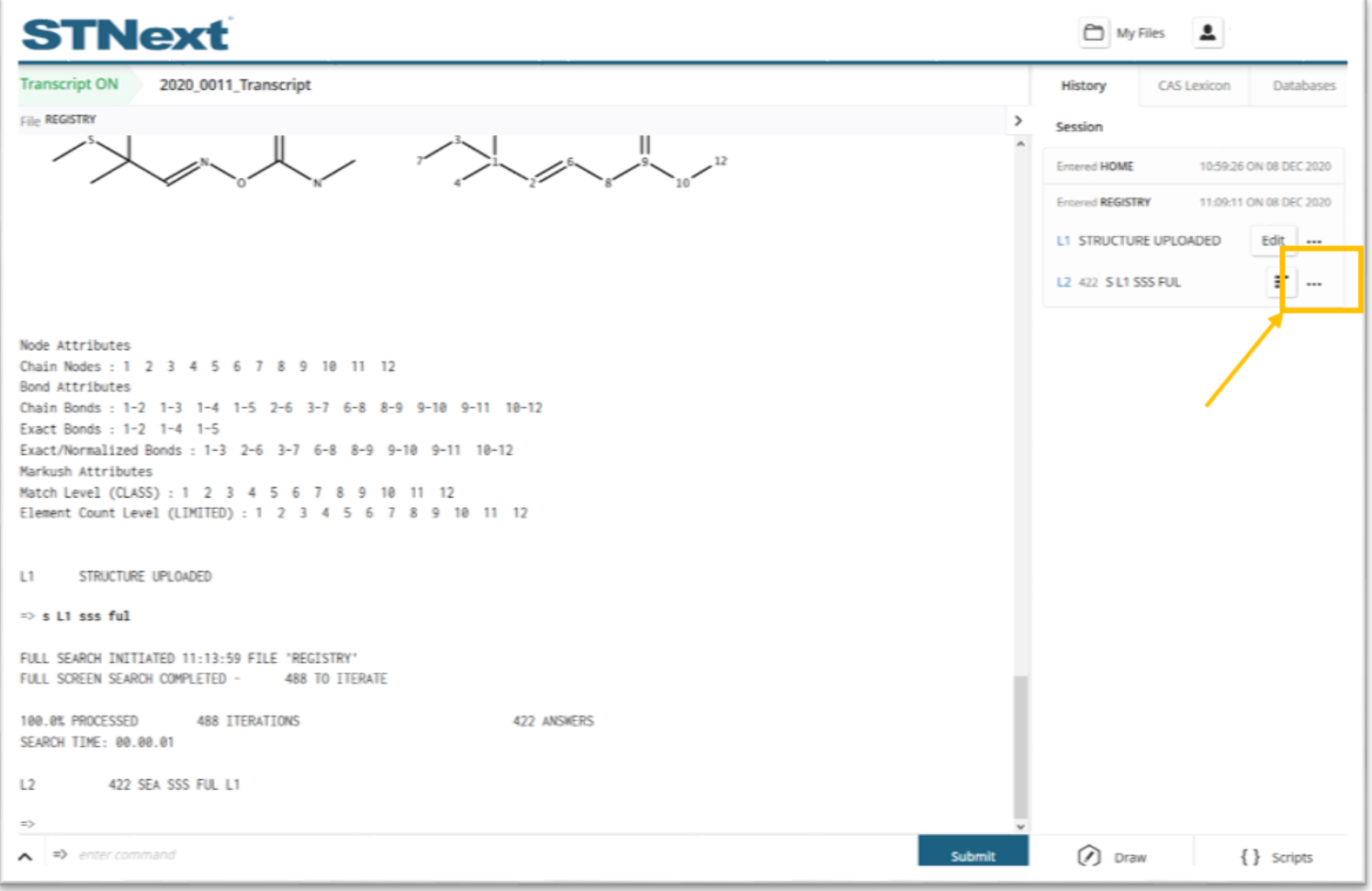
Selecting Create Chemscape Analysis from the ellipses menu kicks off the visualization generation.

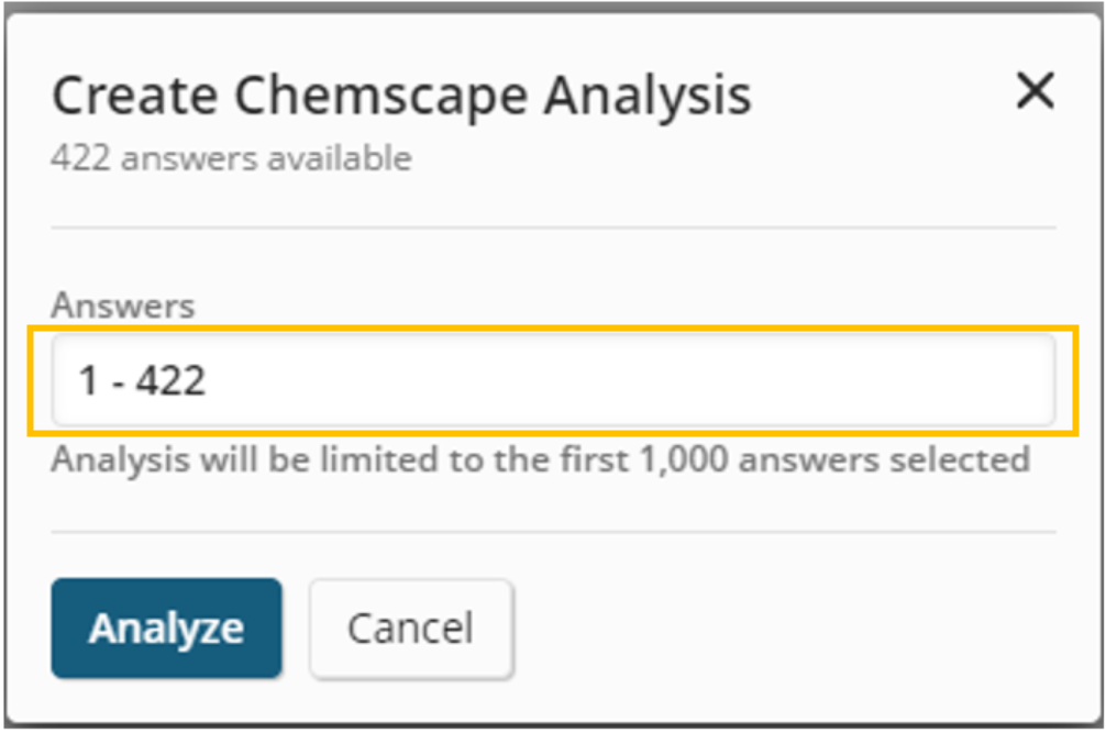
Upon selecting this option, the user is prompted for the range of substances from the results that will be used as part of the visualization.
By default, this will be the first 1000 substances from the result set. The user can also change the selected substances to a different subset of up to 1000 substances. Generating the visualization may take some time depending on the size of the result set to be rendered.
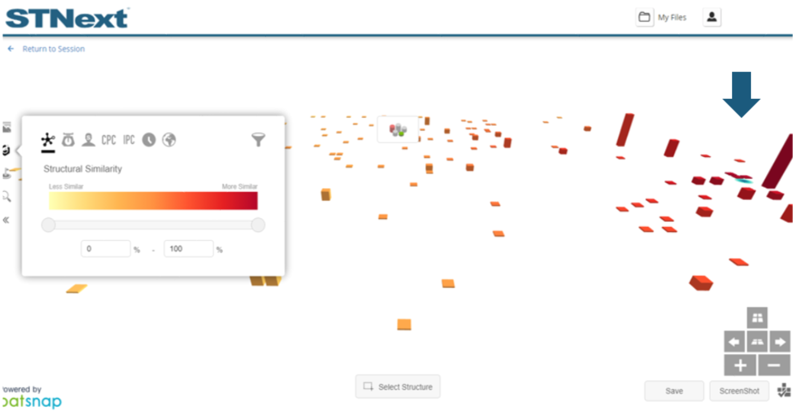
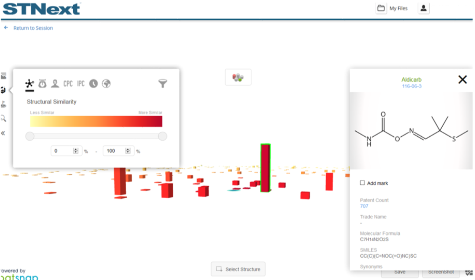
The position of the substances in the presented Chemscape display represents the relative similarity to the substance query and the relative similarity to the other substances that are part of the visualization. The final layout is a best fit when considering the overall similarity or dissimilarity of all substances with each other and the substance query. A blue dot denotes the location of the substance query on the graph.
By default, the substance columns are colored such that substances that are more similar to the substance query are red and substances that are the less similar are yellow. The height of the columns represents the number of patents that reference a given substance.
Users can further explore substances on the visualization by clicking them to get additional information.
For instance, by clicking the tallest substance column, we can explore additional detail about that substance including:
Substance image
Molecular formula
Count of patents referencing the substance
Substance synonyms
SMILES representation
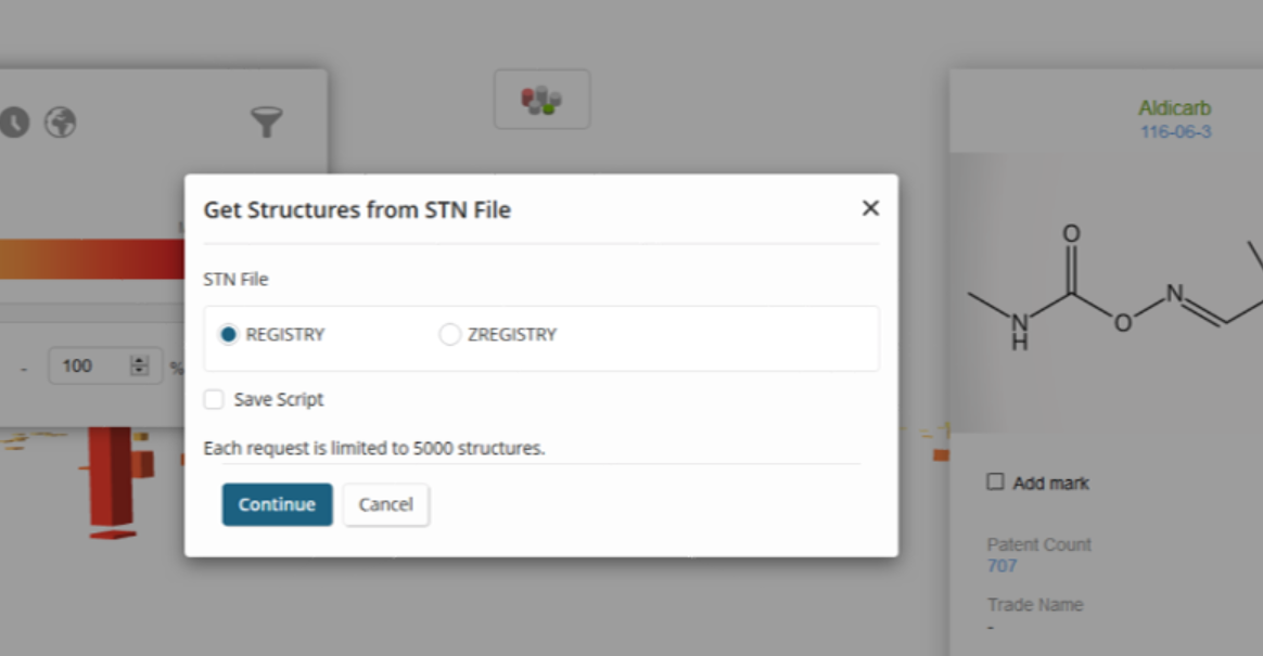
From the substance detail window, the user can crossover to get more information about the substance by clicking the registry number at the top of the dialog.
The user can then select a database for crossover.
The user is then presented with the query results for that related registry number against the selected database.
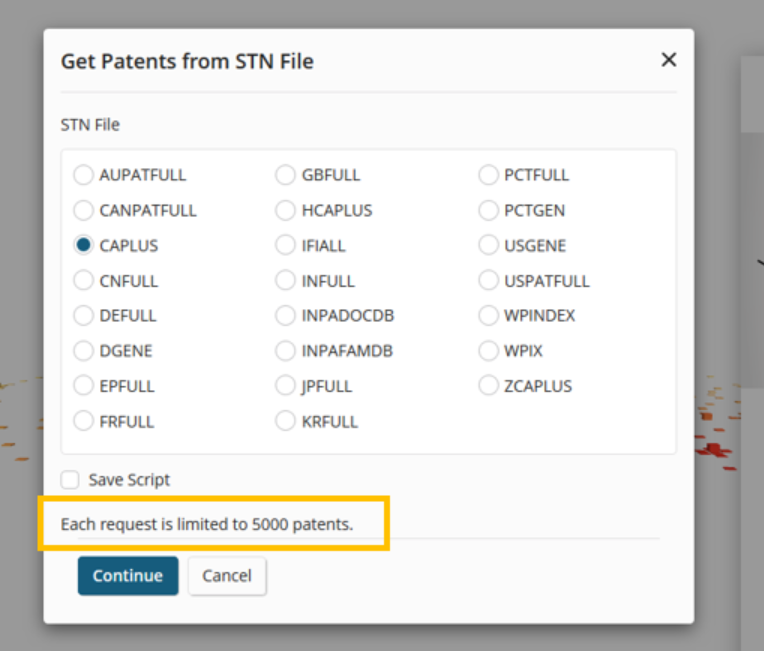
From the substance detail window, users can also explore the patents referencing the substance by clicking the blue patent count.
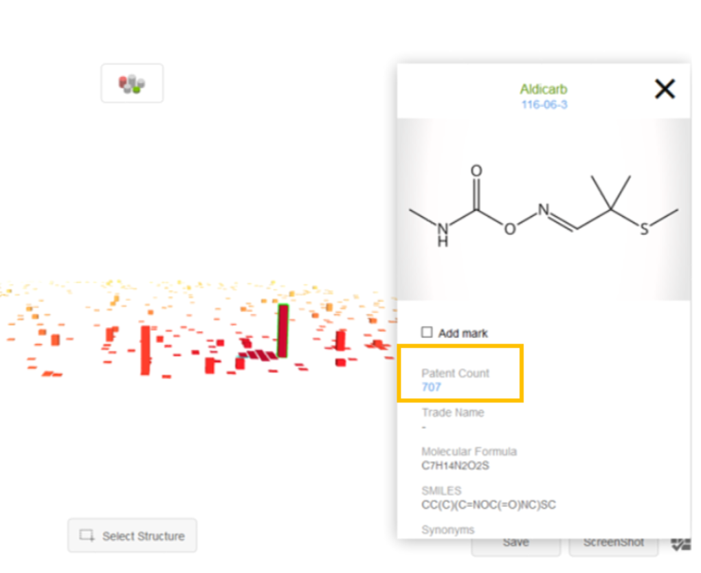
This prompts the user to select a database for crossover. Note that each crossover request is limited to 5000 patents.
The user is then presented with the search results for the related patent numbers.
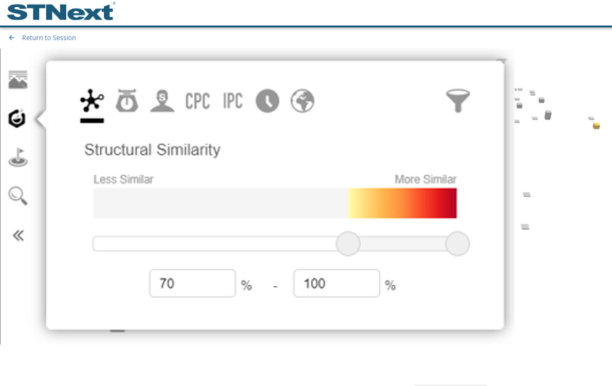
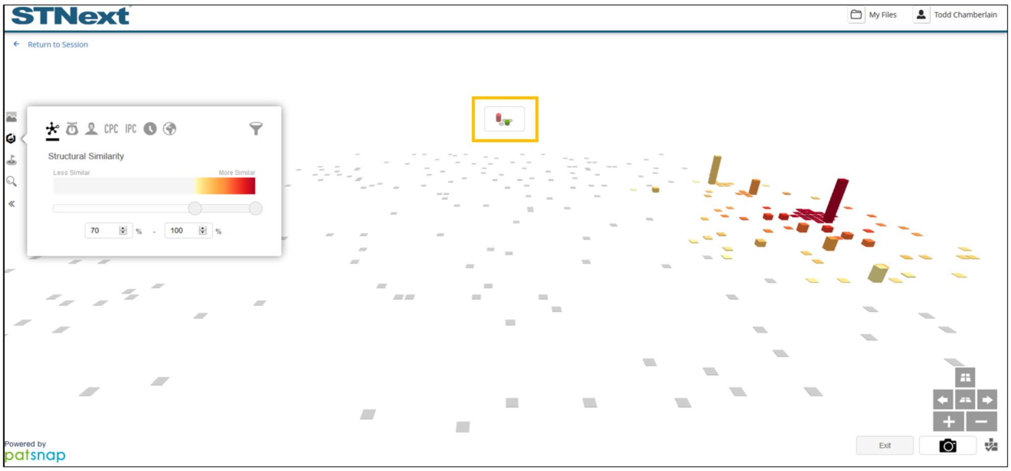
Tools are also available to filter the display to better focus on different factors. For example, the range of similarity represented on the graph can be filtered by using the similarity filter.
For this example, we would click the substance icon on the left, followed by the Structure Similarity icon in the presented window. We could then adjust the lower limit to be 70% (instead of the default of 0); this would focus the graph on higher similarity substances.
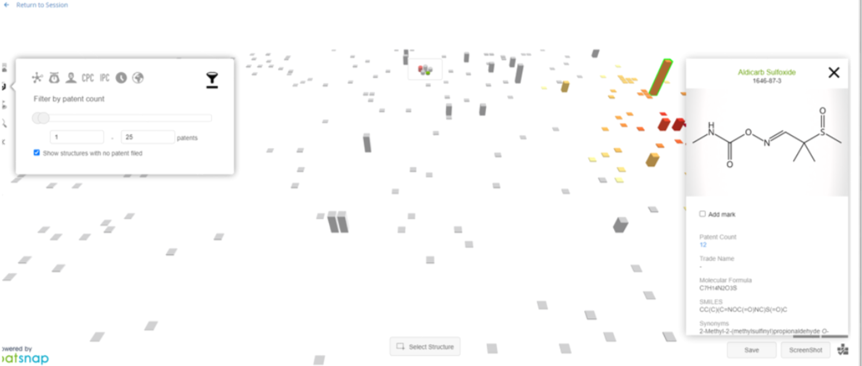
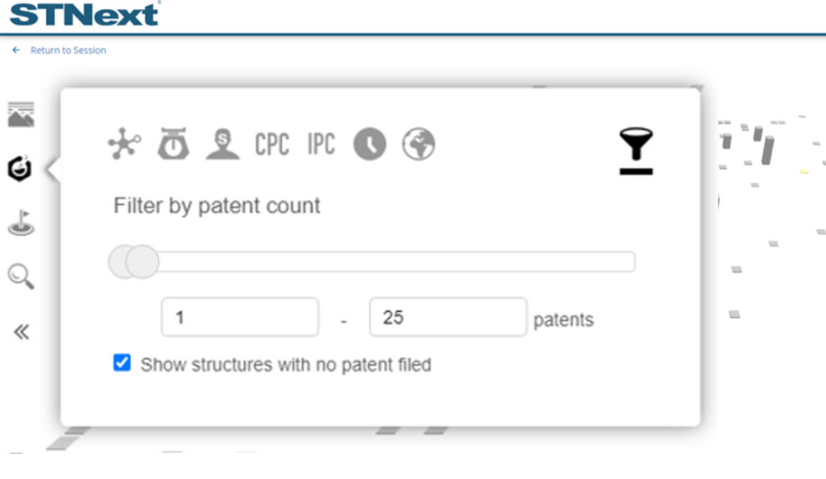
We could also decide to focus on substances with lower patent counts. For example, we would click the substance filter icon on the left, followed by the funnel icon in the presented window. We could then adjust the upper limit to be 25. We could go further by including substances with zero patents by selecting the Show structures with no patent filed box.
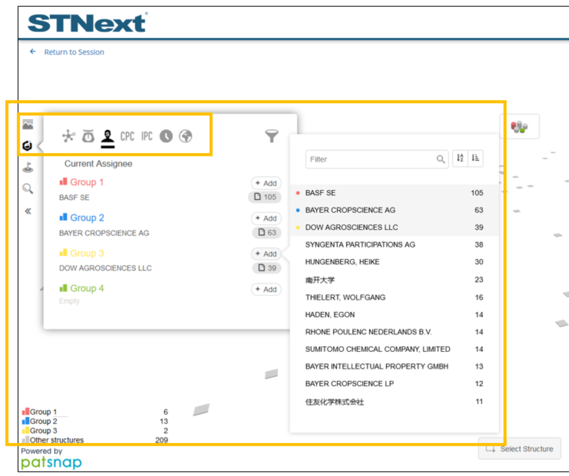
Another filter option available is the patent assignee filter. This filter allows users to identify which substances are associated with patents with the specified assignees.
For example, we would click the substance filter icon on the left, followed by the Assignee icon in the presented window. We can then click the + Add button next to one of the four groups and add the assignees to a group. For this example, BASF, BAYER, and DOW were added to three different groups and the graph now reflects only substances with patents with those assignees.
Note that there are additional filters beyond those that have been described. These include :
Molecular Weight
CPC (Cooperative Patent Classification) Codes
IPC (International Patent Classification) Codes
Publication Year
Jurisdiction
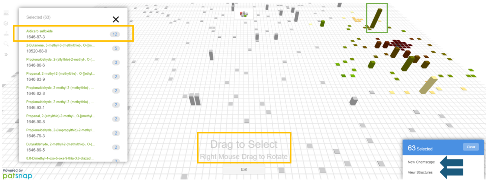
Users can also select a set of structures from the visualization in order to review details about each, view related patents, create a Chemscape visualization with the selected subset, or perform a search for the related substances in STNext.
In the example, we would click Select Structure at the bottom of the visualization, and then click and drag a green square around the target substances. From here, users can click any of the items in the list to get the detail window.
Users can also click the circled number for any item in the list to perform a search for the patents related to that substance.
A visualization with the selected subset of substances can also be created by clicking New Chemscape found in the lower-right corner.
Users can search with the set of selected substances by clicking View Structures found in the lower-right corner. For this example, we will click View Structures.
This prompts the user to select a database for crossover. For this example, we will use REGISTRY.
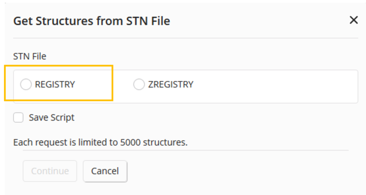
The user is then presented with the search results for the related substances.
Note that this takes the user out of the visualization. To get back to the visualization, go back to the original L number used for the visualization and select Create Chemscape Analysis again from the ellipses (...) menu.
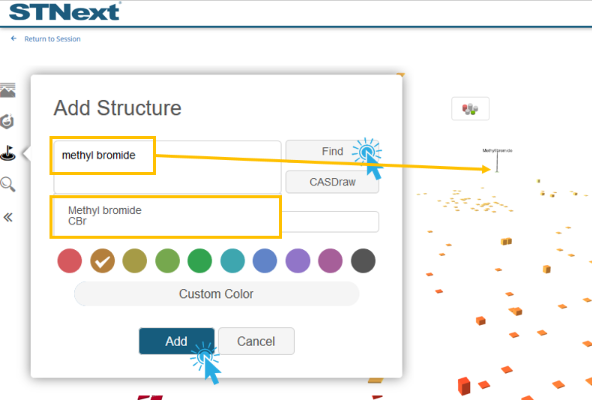
Users can add up to 10 additional structures to the visualization. This provides insight into the relationship between these added structures, the structure query, and the other structures on the graph.
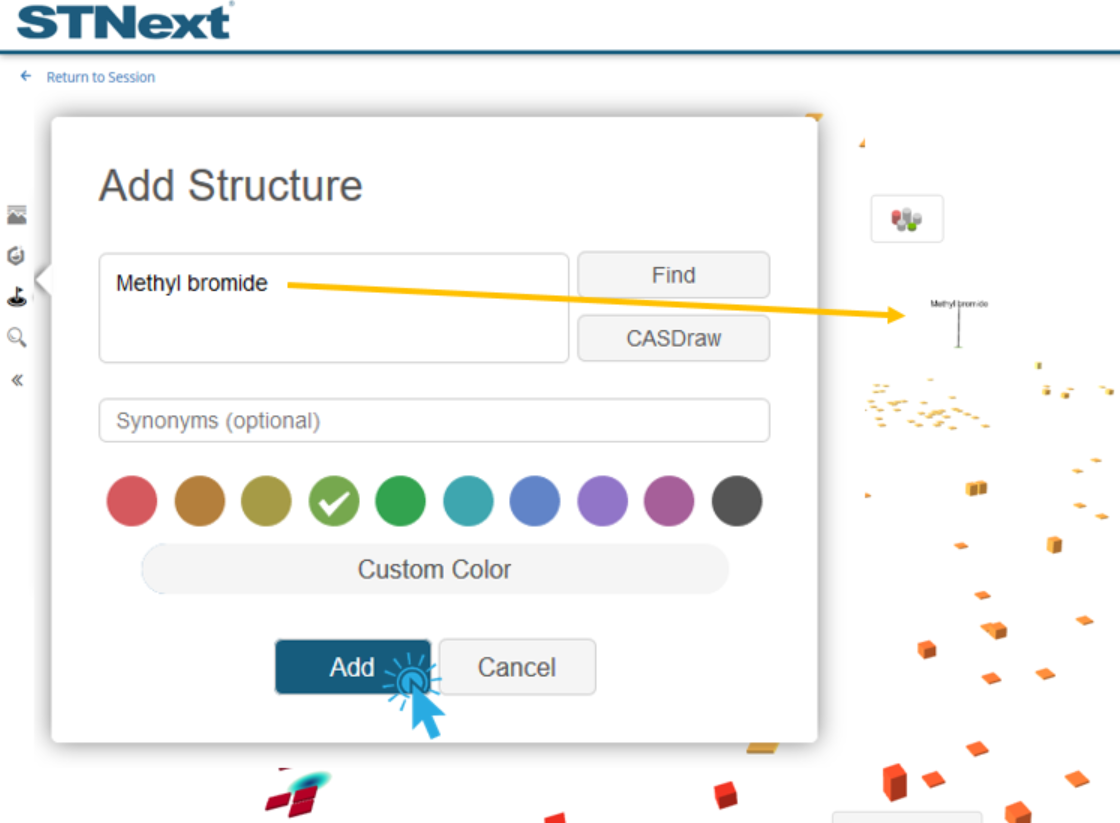
This is done by clicking the Add Structures icon on the left side of the visualization, and then clicking the Add Structure button in the presented window. From here, users can find a structure by entering the name, synonym, or registry number, and then clicking the Find button.
Users can also add structures by drawing them after clicking CASDraw button.

For this example, we will enter the text methyl bromide, and then click the Find button.
We would then select the matching substance from the presented list (up to 5 are presented) and click the Add button.
The selected structure is then added to the visualization, positioning it according to its similarity to the structure query as well as the other structures in the visualization.
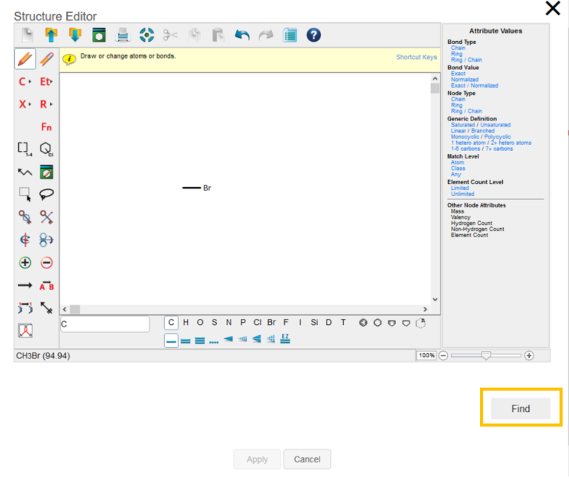
To add a structure via a drawn structure for the example, we would start by clicking the CASDraw button that was mentioned previously.
We would then draw the structure to be searched in the structure editor and click the Find button.
We would then select from the list of matching structures and click the Apply button.
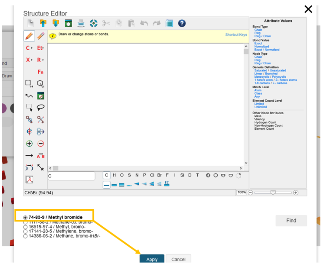
We would then click the Add button. As was seen when adding a structure by name, the selected structure is then added to the visualization, positioned according to its similarity to the structure query as well as the other structures on the graph.
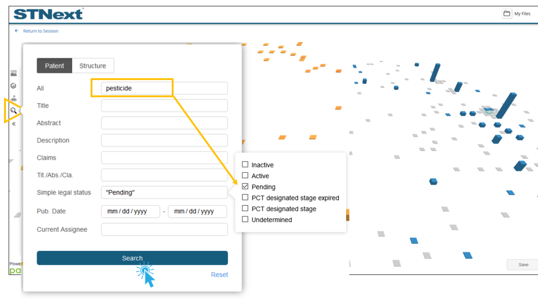
Users can click the Find tool found on the left side of the graph to locate substances using text, publication dates, assignees, and/or simple legal status found in patents which reference a given substance.
For example, a user could enter 'pesticide’ and ‘Pending’ legal status, and then click the Search button. This will then display a list of related substances and update the graph to only show those substances in blue. Users can then click the list or the graph to further explore the related substances.
Users can also locate substances by name, registry number, or by drawn structure by clicking the Structure tab. The functionality is very similar to what was shown for Add Structure.
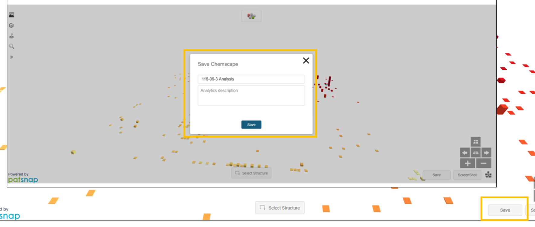
Chemscape visualizations can be saved for future reference by clicking the Save button in the lower right-hand corner of the visualization, and then clicking New Save.
Enter the title and any related description, and then click the Save button.
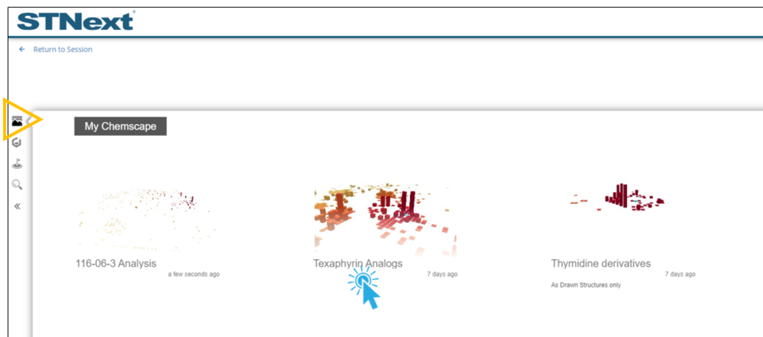
Saved Chemscape visualizations can be reopened by clicking the My Chemscape icon on the upper left, and then clicking one of the listed visualizations.
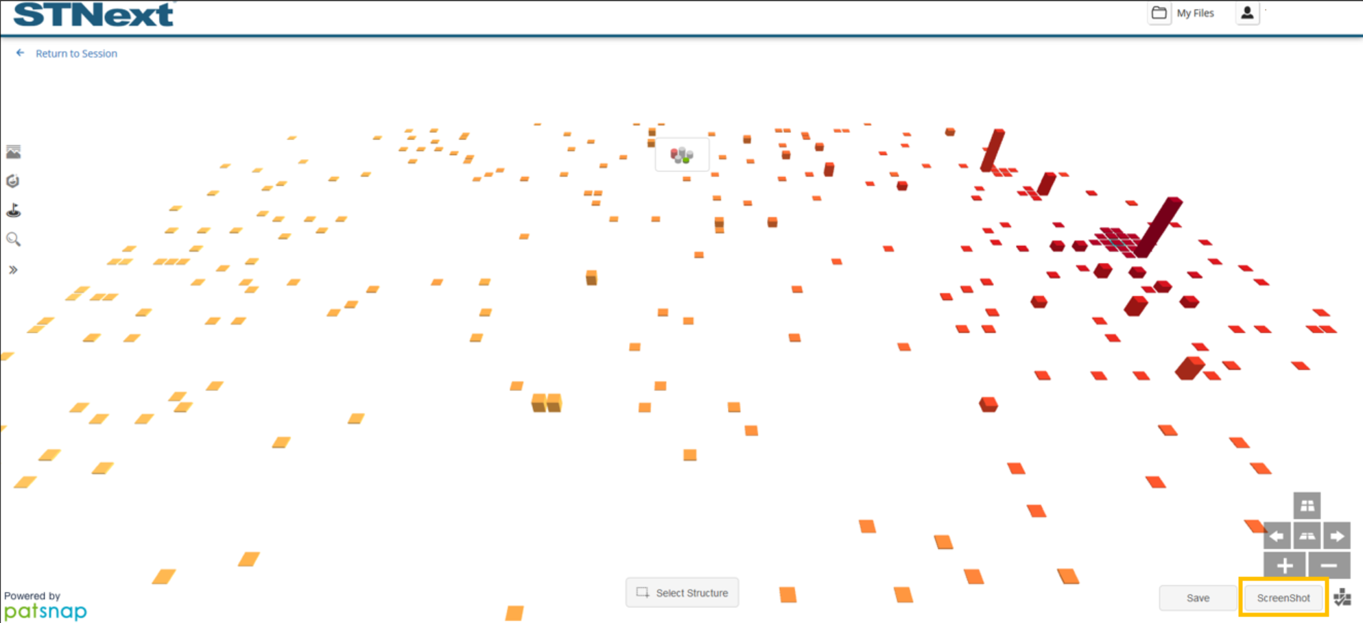
Users can also save a screenshot of the current visualization by clicking the ScreenShot button found in the lower-right corner.
The user can then position the graph as needed and click the camera icon in the lower-right corner when ready. A screenshot is then downloaded to the browser.
Users can also change how the visualization is presented by selecting an option from the view selector found at the top of the visualization.
This can be helpful in focusing on filtered items, and we can see this using the earlier example where the similarity filter was adjusted with the minimum similarity being set to 70%. If we select Highlighted structures only, we can see that the non-highlighted substance columns are flattened.
Other modes include a two-dimensional (2D Overview) representation and a Smooth Height option that defaults to enabled and accentuates patent count differences over the graph.
Back to STN Application Updates